Colocalization
Colocalization is a biostatistical technique to evaluate the evidence that two GWAS share a causal variant at a locus.
Because it evaluates commonality between GWAS signals, colocalization is somewhat similar in spirit to genetic correlation techniques like CT-LDSC. However, whereas genetic correlation evaluates global overlap, colocalization focuses on a single locus. Two GWAS may strongly colocalize at one locus, but not at another. Colocalization techniques facilitate nuanced understanding of where two traits share biological pathways and where they do not.
Colocalization is often paired with Mendelian Randomization, another local technique.
Bayes factor colocalization
Bayes factor colocalization1 is simple, but requires assumptions. It is used as a basis for more advanced colocalization methods.
Data generating model
Assume initially that both traits are quantitative. Assume the following generative model.
- There are \(Q\) genetic variants at the locus of interest.
- We have two GWAS. There are \(N_1\) participants in the first GWAS and \(N_2\) participants in the second GWAS.
- \(y_k\in\mathbb{R}^{N_k}\) is the vector of phenotypes for participants in GWAS \(k\).
- \(G_k \in \mathbb{R}^{N_k \times Q}\) is the genotype matrix for GWAS \(k\) at the locus.
- \(g_{k,i}\in\mathbb{R}^{N_k}\) is the \(i\)th column of \(G_k\).
- \(\beta_{k}\in\mathbb{R}^{Q}\) is the vector of true variant effect sizes for \(k\).
- \(\hat\beta_{k,i}\in\mathbb{R}\) i the GWAS marginal regression coefficient of variant \(i\) in GWAS \(k\).
- \(V_{k,i}\in\mathbb{R}\) is the squared standard error of \(\hat\beta_{k,i}\).
- \(\epsilon_k\in\mathbb{R}^{N_k}\) is the part of \(y_k\) not determined by variants at the locus. \(\epsilon_k\) includes both the environment and other loci.
- \(c_k\) is the number of covariates in the trait \(k\) GWAS model.
Our data generating model is:
We require that \(\epsilon_1\) and \(\epsilon_2\) are independent. This requirement is usually satisfied by assuming that there are no overlapping participants between the two studies.
Category vectors
Variant \(i\) is causal for trait \(k\) if \(\beta_{k,i}\ne 0\). Use \(\mathcal{C}=\{0,1,2,12\}\) to express the 4 disjoint possibilities for any given variant:
- \(0\): The variant is not causal.
- \(1\): The variant is causal for trait 1 only.
- \(1\): The variant is causal for trait 2 only.
- \(12\): The variant is causal for both trait 1 and trait 2.
Call \(\mathcal{C}^Q\) the set of category vectors. Each category vector assigns a causal status to each variant. Assume the causal status of the \(Q\) variants are independent and the probabilities of the four possibilities are \(p_0,p_1,p_2,p_{1,2}\).
Thus, the prior probability of category vector \(c\in\mathcal{C}^Q\) is :
Conditional on variant \(i\) being causal for trait \(k\), we assume the following prior on effect sizes:
for \(\omega_k>0\).
The single causal variant assumption
Let \(\mathcal{A}\) denote the event that at most one variant is causal for each of the two traits. Define the function \(\overline{S}\), whose domain is the set of category vectors corresponding to \(\mathcal{A}\). Define \(\overline{S}(c):=(S_1,S_2)\), where \(S_1\) is the index of the causal variant for trait 1, or 0 if there is no causal variant, and \(S_2\) is the index of the causal variant for trait \(2\), or 0 if there is no causal variant. A pair \((S_1,S_2)\) is called a configuration. There are \((Q+1)^2\) configurations.
Bayes factor colocalization operates conditional on \(\mathcal{A}\), the assumption that at most one variant is causal. This assumption is unrealistic for some loci, but permits significant simplification.
Hypotheses
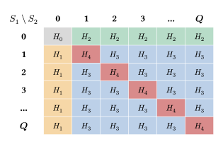
We define 5 hypothesis, which partition the configurations:
- \(H_0\) corresponds to the configurations \(\mathcal{S}_0=\{ (0,0) \}\). There are no causal variants at the locus.
- \(H_1\) corresponds to the configurations \(\mathcal{S}_1=\{ (i,0) : i \ge 1 \}\). There is a causal variant for trait 1 but not trait 2.
- \(H_2\) corresponds to the configurations \(\mathcal{S}_2=\{ (0,j) : j \ge 1 \}\). There is a causal variant for trait 2 but not trait 1 at the locus.
- \(H_3\) corresponds to the configurations \(\mathcal{S}_3=\{ (i,j) : i,j \ge 1 ,i\ne j\}\). Both traits have causal variants at the locus, but they are different.
- \(H_4\) corresponds to the configurations \(\mathcal{S}_4=\{ (i,i) : i \ge 1\}\). The same variant is causal for both traits.
The illustration below shows how the hypotheses partition the configurations.
Configuration odds
Define the following probability ratios:
Let \(h\in \{0,1,2,3,4\}\). Let \(S\in\mathcal{S}_h\). By \((\ref{P_def})\), we have,
Let \(S^0:=(0,0)\). We have
Prior on the hypotheses
We compute the probability of each of the hypotheses. We begin with the unconditional probability, then move the probability conditional on \(\mathcal{A}\).
There is one configuration corresponding to \(H_0\), \(Q\) configurations corresponding to \(H_1\), \(Q\) configurations corresponding to \(H_2\), \(Q(Q-1)\) configurations corresponding to \(H_3\), and \(Q\) configurations corresponding to \(H_4\). Thus, by \((\ref{unconditional_prob})\),
\(\mathcal{A}\) is the union of these disjoint hypotheses. Thus,
Now, compute the conditional probability of the hypotheses.
where we have defined \(\rho_0:=1\) and \(Z:=1+Q\rho_1 +Q\rho_2 +Q(Q-1)\rho_{1}\rho_2 + Q\rho_{1,2}\) and
and where in \((\ref{cond_h_prob})\) we divided the numerator and denominator by \(p_0^Q\).
Marginal GWAS regression coefficients
By the principles of ordinary linear regression, note that the marginal GWAS regression coefficient \(\hat\beta_{i}\) and its standard error \(V_{i}\) are given by
where we have suppressed \(k\), the study-number subscript.
Combining the above implies that
Gaussian integral
The following Gaussian integral will be useful below
It can be proved by standard integration techniques.
Bayes Factor
As the name suggests, a central quantity in the study of Bayes factor colocalization is the Bayes factor. Suppressing the study index \(k\) for now, the Bayes factor for variant \(i\) is defined as
$$ \begin{align} BF(i):=\frac{p(y|S=i)}{p(y|S=0)} \end{align} $$ where \(p\) denotes probability density, and \(\{S=i\}\) is the event that \(i\) is the sole causal variant, while \(\{s=0\}\) is the event that there are no causal variants. Note that both these events are subsets of the event \(\mathcal{A}\) defined above.
Define the quantities
The following result is key:
Proof of result
To prove this, first note that by \((\ref{dg_model})\) we have:
Now take the ratio of the densities of the two distributions. We get
To produce an expression for the Bayes factor, we need to integrate the above over all possible values of \(\beta_i\), weighting by the prior on \(\beta_i\) from \(\(ref{effect_prior})\). We can apply the Gaussian integral from \((\ref{gaussian_integral})\) with
Thus, we have
Note that
and
Combining the above,
as desired
end of proof
To be continued
SUSIE colocalization
todo
Links
Talk on colocalization at International Statistical Genetics Workshop
-
Claudia Giambartolomei, Damjan Vukcevic, Eric E Schadt, Lude Franke, Aroon D Hingorani, Chris Wallace, and Vincent Plagnol. Bayesian test for colocalisation between pairs of genetic association studies using summary statistics. PLoS genetics, 10(5):e1004383, 2014. URL: https://journals.plos.org/plosgenetics/article?id=10.1371/journal.pgen.1004383. ↩